Paradox Data Analysis Tips and Techniques
by Luke Chung, President of FMS, Inc.
Overview
This presentation provides a variety of tips and techniques for using Paradox queries, crosstabs, and graphs to analyze and present data. Some
ObjectPAL techniques are presented, but extensive knowledge of ObjectPAL is not necessary to understand most of the presentation and paper. These topics are covered:
Advanced Query Analysis
The following are a few examples of using queries to generate advanced results. No programming is required for these techniques. Three common needs
are covered:
Frequency distributions reveal the number of records that contain values within numeric ranges. In this example, we want to know how many patients
fall into different age categories (under 25, 25 to 40, 40 to 50, 50 to 60, and 60+). A simple two table query calculates these results even when the size of the numeric ranges are not identical. In
this example, we use two tables: Age_Grp.DB for age groupings and Patient.DB for patient data. The frequency distribution query is called FreqDist.QBE. Just follow these simple steps:
Step 1: Create a table defining the groups and numeric ranges
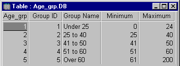
Simply create a table with four fields: Group ID (counter), Group Name (text), Minimum (number), and Maximum (number). For each record, define the
groups and its low and high values:

Notice how the [Maximum] value of one record is smaller than the [Minimum] value of the next record. They cannot be identical or else border values
would fall into two groups. In our example, the Age data are integers so using integers in this table is okay. Otherwise, you can use numbers very close to each other (e.g. 24.9999999). You can name
and specify as many groups as you like.
Step 2: Create a multi-table query
Create a query with the data table and the group definition table defined above:
Query
 ANSWER: :PRIV:ANSWER.DB

 Age_grp.DB | Group ID | Group Name | Minimum | Maximum |
            | Check    | Check      | _minVal | _maxVal |

 Patients.DB | ID                    | Age                  |
             | calc count as "Count" | >=_minVal, <=_maxVal |

EndQuery
The first two fields in the query results come from the group table: the [Group ID] field (which controls the sort order), and the [Group Name]
description. The third field is the count of the Patient (data) table's [ID] field (this field is used since it exists for every record). The final field defines the link between the two tables. Using
the Patient table's [Age] field, the criteria is ">= _minVal, <= _maxVal". This "bins" the Patient data into the age groups defined by the Age_Grp table.
Step 3: Run the Query
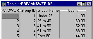
Running the query provides the desired results:

Be careful about sorting if you have text fields defining the groups. In this example, if the Group table's [Group ID] field is not used in the query
(Checked), the results would be in Ascending order by [Group Name] and "Under 25" would be the last record.
The example shown is very simple. In addition to counting records, you may also want to perform other analysis. For instance, you may want the Count
and Average Cholesterol for each age group. Simply put "calc average" in the [Cholesterol] field, and you'll get the results.
You can also show frequency distributions for multiple groups in one query. For instance, you may want to see the count by state. Just add a Check to
the [State] field, sort by State and Group ID, and each state's frequency distribution is shown.
Another application of this technique involves the use of date fields in financial analysis. For instance, you can define the date ranges of fiscal
quarters in the grouping table, and use that to query against financial tables for the results summarized by quarter. (Quarters, in accounting, often don't fall on the last day of each month).
For a field, calculating the percent of each record to the total for an entire table (or group of related records) is useful for determining the
relative size of each record. This is achieved by using two queries. The first sums the total of each group, and the second compares each record to the total.
In this example, we use the [Cars] table containing sales data by brand for each year; and two queries: Car_Sum.QBE and Car_Pcnt.QBE. Here's how they
work:
Step 1: Create a Query calculating the Totals and Run it
This is a simple query that sums the values by year:
Query
 ANSWER: :PRIV:ANSWER.DB

 Cars.db | Year  | Sales             |
         | Check | calc sum as Sales |

EndQuery
This generates an Answer table with two fields (Year and Sales) and a record for each year.
Step 2: Create a Query with the Totals and the Original Table
This is a simple select query that retrieves fields from the Cars table and creates a new field for the Percent of Total calculations. The Cars table
is linked on the [Year] field to the Answer table generated in the previous step.
Query
 ANSWER: :PRIV:ANSWER.DB

 FIELDORDER: CarsNorm.db->"Year", CarsNorm.db->"Company",
             CarsNorm.db->"Sales", 4

 SORT: CarsNorm.db->"Year", CarsNorm.db->"Sales" DESCENDING,
       CarsNorm.db->"Company", 4

 CarsNorm.db | Company   | Year         |
             | CheckPlus | Check _join1 |

 CarsNorm.db | Sales                                             |
             | CheckDescending _s, calc 100*_s/_total as Percent |

 :PRIV:Answer.db | Year   | Sales  |
                 | _join1 | _total |

EndQuery
The query was manually modified to display fields in the desired order, and records in descending sales (percent of total).
Step 3: Run the Query
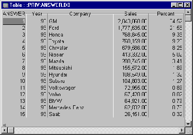
Running the query provides the desired results:

The percent field shows values ranging from 0 to 100. An alternative is to show percent as a value between 0 and 1; however, since Paradox by default
shows numbers with 2 decimal places, it is easier to use the scale 0 to 100 to display more significant digits.
The example shown works very easily. Unfortunately the same technique cannot be used if you do not have a group field (like [Year]). If your first
query totals the whole table and provides one record, you cannot link that value in a query to another table. However, you can just copy the value and paste it directly into your query's equation.
Paradox queries easily link records across multiple tables where field values match. There are situations where non-matching fields are required. The
use of outer join queries allows the selection of all the records from one table regardless of a corresponding match in another table.
A related request is the determination of records that are "not in" another table. A simple variation of an outer-join query does the trick:
Query
 ANSWER: :PRIV:ANSWER.DB

 SUBSET.DB | Company         |
           | _join1, count=0 |

 CARS2.DB | Company           | 1993      | 1994      |
          | CheckPlus _join1! | CheckPlus | CheckPlus |

EndQuery
In the example above, the SUBSET table contains a small list of companies. The CARS2 table contains sales information for all companies. The query
retrieves the records from the CARS2 table that are not in the list of companies in the SUBSET table. The outer-join is from the CARS2 table (since it is the complete list), and linked to the SUBSET
table with a "count=0" criteria.
Query Restarts
When the underlying tables of a query are modified by another user, Paradox can restart the query. In the header of each table is a counter that
increments when a record is modified. As Paradox runs its query, it occasionally looks at this header section, and if the number changes, the query restarts. In high transaction environments with
large tables, queries could potentially never complete. The idea behind this behavior was that the ANSWER table (when you got it) would always be correct; that it would always contain consistent data
valid at one point in time. Unfortunately, a query that never completes is pretty useless. Fortunately, Paradox offers ways to avoid query restarts, and in many cases runs much faster.
Query Options: Table Update Handling
While designing the query, there are three choices. Under Paradox 7, the choices are in the Query menu:

For Paradox 5, the choices are under Properties|Query Options:

The first option forces Paradox to restart the query if the table changes. The second option places a lock on the tables to prevent modifications
from others during the query. This is very disruptive behavior and not acceptable in most multi-user cases. The final option does not impose table locks and does not restart if changes occur during
the query. This allows "dirty" reads which can cause incorrect results, but the query always completes in one pass. Unless key fields are allowed to be modified, dirty reads are generally acceptable.
In these cases, the answer may not be up-to-date, but was correct at a point in time.
Watch Out!
If key fields are modified, dirty reads can miss or double count records that "jump" in the table during the query. The answer in this case is not
only incorrect, but was never correct at any point in time. For instance, imagine a query processing a keyed table. As it goes down the table, it passes a record that is edited and posted before the
query completes. If the key field is modified to cause that record to "jump" below the query, the query will read it again when it gets to it. Even with a simple "calc sum" query, the answer in this
situation is not only out-of-date, it is completely wrong since the record was double counted. Similarly, if changes cause a record to jump "up", the query could miss it completely. Depending on your
situation, suspending query restart may or may not be appropriate.
Once queries generate the results you want, you want to present it in a report. In multi-user environments, the table containing the data for the
report should be in the user's private (:PRIV:) directory. This prevents problems if multiple users are running the same report. There are several ways to use reports:
Simply create a report based on the ANSWER table. This works and even handles multi-user situations since the ANSWER table is always in each user's
private directory.
Unfortunately, this method is problematic. If the current ANSWER table does not have the same structure as the report, it is not possible to properly
modify the report. This means you can only modify the report right after generating the ANSWER table.
Unlike the previous method, rename the ANSWER table to another table in the private directory prior to creating the report. This way, as long as the
temporary table is not deleted or replaced, the report can be opened and modified. To automatically have the report deleted whenever you exit Paradox, name the table with two leading underscores (e.g.
"__Table.DB").
Alternatively, you can keep the table in the private directory and place the results of your query (or queries) into it by using an INSERT query.
There are occasions when reports based on one table need to be based on data in another identically structured table. If the report is based on a
table in the private directory, the solution is simple (just replace the current table with the desired data). However, you may not want to replace the current table. The solution is to switch the
source.
Using Table Aliases
When creating a report, tables are added to the report's Data Model. In the Data Model, each table should be given an alias (right click on the table
object). This way, the fields placed on the report reference the alias rather than the actual table name. If a new table needs to be used, modify the report's data model, add the new table, delete the
existing table, and set the new table's alias to the old table's alias. The report automatically uses data from the newly referenced table. Unfortunately, you cannot do this programmatically through
ObjectPAL. However, with ObjectPAL, it is even easier to change the main table of a report and no modification of the report is necessary.
Use the ReportOpenInfo Record Type
With a little ObjectPAL, you can easily change the master table of a report (or form) with the ReportOpenInfo variable (record) type. Rather than
opening the form directly, use a variable of ReportOpenInfo type and set its Name and MasterTable elements. The method below shows how to open any report with a specified table.
method ReplaceReportTable(strReportName string, strDataTable string)
  var
    r  report
    ri ReportOpenInfo
  endvar
  ri.Name = strReportName
  ri.MasterTable = strDataTable
  r.open(ri)
endmethod
See the on-line help system for the Open command for more details. Instead of specifying the MasterTable, you can specify a QueryString and base the
report directly on that. This eliminates the need to separately execute the query (and create an ANSWER table). Paradox automatically creates its own private table and bases the report on that.
By using the ReportOpenInfo technique, you can create a report based on a table stored in a template directory rather than relying on the temporary
ANSWER table. That way you can always modify the report in design mode. When you use the report, link it to the table in the private directory. When using this technique, a message to save the report
appears when you try to close it. To avoid this confusing message for users, use a delivered report (*.RDL).
NOTE: A similar record type, FormOpenInfo, is available for forms.
Crosstabs are a powerful tool for summarizing data and showing relationships between three fields. A crosstab is basically a matrix displaying data
from a query with 2 Check fields and one summary (e.g. CALC SUM, CALC COUNT, etc.) field. This format is most familiar to spreadsheet users and is a useful way to convert normalized data into
un-normalized form and can reveal hidden relationships in large data sets.
Parts of a Crosstab
There are three parts to a crosstab:
Column Field
Every unique value in the column field becomes a field in the crosstab
Categories (Row) Fields
One or more category fields form the left side of the matrix. Each unique combination of values in the category fields is a separate record in the
crosstab.
Summary (Value) Field
The summary field is the data that is summarized for the matrix. The summary types can be Count, Sum, Min, Max, or Average. The results are displayed
in the "cells" of the matrix.
Creating Crosstabs Interactively
Crosstabs can be easily created in a form by selecting the crosstab object, placing it on the form, and specifying the column, categories, and
summary fields under the Define Crosstab option when right clicking on the object. You can also specify the summary type. When you run the form, the crosstab is calculated and displayed on the form.
If your columns or records exceed the space provided, you can scroll through the crosstab. If you chose multiple categories, the combination of the categories are shown in the left most column.
Once a crosstab is created on the form, it can be converted to a table using this command:
xtab.action(DataSaveCrosstab)
where xtab is the name of the crosstab object. This creates a CROSSTAB.DB file in your private directory.
Using Crosstabs Programmatically
If you need to move around the crosstab programmatically, you can use the CurrentRow and CurrentColumn properties to move to the cell you want. The
rows and columns are integers (smallint) that identify each cell.
Using Crosstabs in Reports
If you have a Crosstab table, creating a report for it is just like any other table. However, if you want to create a report for repeated use based
on the results of a crosstab, it can be quite tricky. The problem is you may not know what the crosstab's field names are going to be. If a new value exists in the Column field, or an existing value
is removed, the fields in the Crosstab table are different.
Finally, if you have too many fields (too many unique values in the column field), your data may not be able to fit on one page. Other than going to
smaller and smaller fonts, and using Landscape mode, there's not much that can be done to add width to your paper.
The easiest approach to creating a crosstab report is to create a form with a crosstab then open and save it as a report. When the data changes, the
crosstab automatically adjusts in your report. If you base a report on the crosstab table, this feature is not available and you will have to programmatically add or remove fields from your report
(very painful code).
Graphs are a very powerful way to display data relationships in Paradox tables. Paradox graphs are very well integrated and offer instantaneous views
of your data just like a table frame. For instance, for a regular graph, if the underlying data changes (even across a network), the graph immediately updates to reveal the new data. Similarly, graphs
can be linked in a one-to-many relationship that allows different views of detail records as the master record changes. Extremely powerful.
There are several graph types many with 2 dimensional and 3 dimensional options:
|
XY
Line
Rotated Bar*
|
Stacked Bar*
Bar*
Area*
|
Columns*
Pie*
|
Surface (3D)
Ribbon (3D)
Step (3D)
|
*Both 2D and 3D options
3D graphs have a depth dimension and can be very appealing. The 3D Pie graph is much nicer than its 2D cousin. Other 3D graphs also work particularly
well for small data sets (few X axis categories). Unfortunately, many of the 3D graphs are unusable with larger data sets where the X-Axis labels are so close that they overlap and become unreadable.
The XY and 2D graphs grow to the size of the graph object you create. 3D graphs are designed to fill a square.
Hints for Using 3D Graphs (excluding Pie graph)
Do not set X-Axis to Alternate ticks. In 2D graphs, cramped X-Axis labels are more readable when they reside on alternate rows. In 3D graphs, setting
Alternate only makes the graph smaller, which worsens the situation.
If Legends are used (only possible for Area, Ribbon, Rotated Bar, and Stacked Bar graphs), the legend should be on the side with more space. In our
examples where the horizontal dimension is larger than the vertical, placing the legend on the right side does not affect the graph size. Placing it below the graph shrinks the graph and wastes empty
space on the side.
When creating a graph, three Data Type options are available: Tabular, 1-D Summary, and 2-D Summary. Note that these are not related to
the 2D and 3D graph types. This is a summary:
|
Data Type
|
Description
|
Example with a Bar Graph
|
|
Tabular
|
Each record is one data item
|
The bar graph shows a separate bar for the sales of each product each year. One bar per record.
|
|
1-D Summary
|
Data for each unique X field value is shown with its sum of the Y field
|
The bar graph shows for each product (X) total sales (Y) across all years. One bar for each product.
|
|
2-D Summary
|
Data for each unique X field value is shown with the sum of its Y field in the group field components
|
With [Year] as the group field, the bar graph shows for each product (X), the total sales for each year (Y),
where each year is a separate bar.
|
Tabular graphs always update when the underlying data is modified. When a 1-D or 2-D Summary graph is added to a form on its own (as the
master table), it does not refresh when its underlying data is modified. However, when it is added as a detail form, it updates whenever the master record or detail records are modified.
This section describes how to use ObjectPAL to create a new form with a graph of any table. This is a bit complicated, but can be used to use a graph
for any data set. In most cases where you know the table and fields you want in your graph, it is simpler to interactively create a graph and only use ObjectPAL to adjust the properties necessary when
you run it.
This example shows how data from two tables linked in a one-to-many relationship can be displayed. The graph is based on the detail table and changes
as one scrolls through the master records. The sample data is a result of a regression and shows for each data point the actual X and Y values, plus the estimated (regression) Y. An XY Graph is
generated with the X field forms the X-axis, the Y value the scatter plot, and the estimated Y the regression line. (Sample in OPAL.FSL).
The important ObjectPAL commands in the example below are:
| Method/Property |
Purpose |
| Create |
Creates a form or UIObject on a form.
When creating a UIObject, the object type is specified. A graph object is called a ChartTool as opposed to GraphicTool which is a graphic object (BMP)
|
| dmAddTable |
Adding table to a form's data model |
| dmLinkToFields |
Defining the link fields between two tables in the data model |
| XAxisName |
Assign the X field to this property |
| SeriesName |
Assign the Y field to this property (based on value of CurrentSeries) |
| MethodSet |
Add a method to a form/object |
ObjectPAL Graph Example
Paradox offers several ways to use queries in ObjectPAL. Use the ExecuteQBE() command to run a query defined in a QUERY..ENDQUERY statement, or use
it in combination with the ReadFromFile() command to use a saved QBE statement. Similarly, if you are using a SQL string rather than QBE, use the ExecuteSQL() command.
With either ExecuteQBE() or ExecuteSQL(), the results can go to an output table (ANSWER) or a TCursor. A TCursor can be much quicker and simplifies
the processing of the results since you already have a handle to the results.
Sometimes you don't know the tables, fields, and criteria in advance, so a saved QBE or SQL file is not possible. In these situations, you need to
create a query programmatically. The easiest is for setting criteria or field names by using a tilde variable (~variablename) in the saved query. The tilde variable is replaced by the variable's value
when the query is run.
In a more general situation where you do not know the number of fields or tables and how they link, it is not possible to use this technique. You
must create a query string or SQL string programmatically and use the ReadFromString() command before executing it. There are many ways to do this:
Creating Queries Programmatically
The brute force method is to create the entire QUERY..ENDQUERY string in a variable by concatenating pieces of it. This is a rather painful process
where each line of the query is built piece by piece, including carriage returns (\n), and field separators (|). Here's an example where the "Stock No" is based on the current value of a TCursor:
var
  qs string
  qVar query
endvar
qs = "Query\n\n" +
     ":sampData:Lineitem|Order No|Stock No |\n" +
                       "| _ordNo |" + tc."Stock No" + "|\n\n" +
     ":sampData:Orders|Order No|Customer No |\n" +
                     "| _ordNo |_cust       |\n\n" +
     ":sampData:Customer|Customer No|Name  |Phone |\n" +
                       "| _cust     |Check |Check |\n\n" +
     "EndQuery"
qVar.readFromString(qs)
qVar.executeQBE()
Of course, the example above is trivial (it could have easily used a tilde variable); however, using a string could easily allow the joining of
several tables together based on other criteria.
Using Query Methods in Paradox 7
In Paradox 7, a several new commands make programmatic query development much easier. These commands apply to a variable of query type and allow
manipulation of the query in a more object oriented manner. These are the most important new commands (for a complete list, look under "Query Type" in the on-line help system):
| OPAL Command |
Definition |
| AppendTable |
Adds a table to the current query |
| AppendRow |
Adds a row to the current query |
| CheckField |
Check a field |
| CheckRow |
Check an entire row (all fields in the table) |
| ClearCheck |
Remove check |
| SetCriteria |
To set the criteria for a particular table's field |
| InsertTable |
Add a table before the current query |
| InsertRow |
Adds a row before the current row |
| RemoveTable |
Remove a table |
| RemoveRow |
Remove a row |
| CreateAuxTables |
Set whether auxiliary tables are created (Changed, Inserted, Deleted, etc.) |
| SetRowOp |
To designate row operations (Delete, Insert, Set) |
Here's a simple example selecting all the Customers in DC or VA:
tableID = qVar.AppendTable("CUSTOMER.DB")
rowID = qVar.AppendRow(tableID)
qVar.SetCriteria(tableID, rowID, "State", "DC or VA" )
qvar.CheckRow(tableID, rowID, CheckPlus)
if qVar.isQueryValid() then
  qvar.ExecuteQBE()
else
  errorShow()
endif
This section provides some examples of using ObjectPAL for data analysis:
Each record can be provided with a cumulative sum by calculating the sum from previous records and incrementing the value(s) from its record. This is
a very simple task with a scan loop through the table. A common application is an accounting ledger that calculates a balance (cumulative sum) based on the list of credits and debits:
const
  strLedgerTable = "Ledger"
endconst
var
  tc TCursor
  numBalance number
  tv TableView
endvar
tc.open(strLedgerTable)
tc.edit()
numBalance = 0
scan tc :
  numBalance = numBalance + tc."Credit" - tc."Debit"
  tc."Balance" = numBalance
endscan
tc.endedit()
tc.close()
A rank value for each record provides an way to identify its place among many records. While reports can view the data in sorted order, a rank value
is useful when data is shown in one sort order and you want to identify each record's ranking based on another sort order (for instance, company rank based on sales, but shown in alphabetical order).
Assigning rank values for each record is a relatively simple task. With the data sorted in the desired order, you can easily assign an incremental
value to each record. An extra complication is for tied records which must be assigned a rank order based on the average rank of tied records. For instance, if the 3rd through 6th
records hold the same values, they are all given a rank value of 4.5.
This example includes two methods that are on the CODE.FSL form. The first creates a table sorted in the desired order; the second performs the rank
calculation:
method pushButton(var eventInfo Event)
  const
    strDataTable = "Patients" ; Table with original data
    strSortTable = "Sort"     ; New sorted data
    strSortField = "Age"      ; Field to sort
    strRankField = "AgeRank"  ; Field to place ranking results
  endconst
  var
    dataTbl table
    tc TCursor
    strSql string
    sqlVar SQL
    tv TableView
  endvar
  dataTbl.attach(strDataTable)
  sort dataTbl on strSortField to strSortTable endsort
  if tc.open(strSortTable) then
    RankValues (tc, strSortField, strRankField)
    tv.open(strSortTable)
  endif
endmethod

; Fills in the strRank field based on values in the strData field.
; INPUT: SortDataSet Recordset assumed to be sorted in rank order.
;        strData Field with data to rank.
;        strRank Field to place rank value.
method RankValues (var SortDataSet TCursor, strData String, strRank String)
  var
    x, lngRank, lngRecs, lngTies longint
    dblCurr, dblAvgRank, lngWeight number
    NewRank_b, ok_b logical
  endvar
  lngRank = 0 ; Current rank value.
  SortDataSet.Home()
  SortDataSet.Edit()
  While Not SortDataSet.eot()
    dblCurr = SortDataSet.(strData).value ; Set current value.
    NewRank_b = False
    lngRecs = 0           ; Number of records in current ranking.
    lngTies = 1           ; Number of tied records
    lngRank = lngRank + 1
    ; Determine number of records with the next rank value
    while TRUE
      ok_b = SortDataSet.NextRecord()
      If ok_b Then
        NewRank_b = (SortDataSet.(strData).value <> dblCurr)
        lngRecs = lngRecs + 1
        If Not NewRank_b Then
          lngTies = lngTies + 1
        endif
      endif
      ; Loop until the end of the table or a new value is encountered.
      if not ok_b Or NewRank_b then
        quitloop
      endif
    endwhile
    if lngTies = 1 Then ; Only one unique record
      lngWeight = lngRank
    else ; Calc average rank for multiple records
      lngWeight = (2 * lngRank + (lngTies - 1)) * lngTies / 2
    endif
    lngRank = lngRank + (lngTies - 1)
    SortDataSet.skip(-lngRecs) ; Go back to first record of group.
    if not ok_b then
      lngRecs = lngRecs + 1
    endif ; Handle last record.
    dblAvgRank = 1.0 * lngWeight / lngTies
    For x from 1 To lngRecs
      SortDataSet.(strRank).value = dblAvgRank
      SortDataSet.NextRecord()
    endfor
  endwhile
  SortDataSet.endedit()
endmethod
To perform the ranking on the original table (without creating a separate sort table), create a secondary index on the desired field, open a TCursor
using the index, and run the RankValues method.
With rank values it is also easy to identify each record's percentile. By definition, the first and last records are percentiles 0 and 100. Knowing
the maximum rank (may be less than the total number of records if multiple records have the maximum value), the percentile of each record is 100 times its rank minus one, divided by the maximu rank
minus one.
This example is from the Percentile button on the CODE.FSL form and uses the results from the previous step:
method pushButton(var eventInfo Event)
  const
    strDataTable = "Sort"
    strRankField = "AgeRank"
  endconst
  var
    q query
    tbl table
    maxRank number
    tv TableView
  endvar
  tbl.attach(strDataTable)
  maxRank = tbl.cmax(strRankField) ; Get maximum rank value
  q = Query
        ANSWER: :PRIV:ANSWER.DB
        SORT.DB | AgeRank | AgePercentile                       |
                | _rank   | changeto 100*(_rank-1)/(~maxRank-1) |
      EndQuery
  if q.executeQBE() then
    tv.open(strDataTable)
  endif
endmethod
Moving averages are usually calculated for time dependent data to smooth out short term variations. A classic example is stock prices. People use a
variety of moving averages (10, 30, 200 days, etc.) and compare the current price against them. Basically, a moving average for a particular day is the average price over the previous x days, where x
is the number of days in the moving average.
There are many ways to calculate this in Paradox, one way is to sort the data by date, and scan the results. An array of values for the number of
records in the moving average (say 10 days) is maintained. After the first 10 records are retrieved, the first average is calculated. With the 11th record, the first value is replaced by
the new value, and a new average calculated, and so on. This example comes from the CODE.FSL form and calculates the 10, 30 and 100 day moving average for Borland's stock price as stored in the
BORLAND.DB table. A form, BORLAND.FSL shows this data graphically.
const
  strTable = "Borland"
  maxDays = 100
endconst
var
  tc TCursor
  ar array[] number
  recs, aryIndex, x, idx smallint
  sum10, sum30, sum100 number
endvar
tc.open(strTable)
tc.edit()
ar.setsize(maxDays) ; Create array of last 100 records
recs = 0
aryIndex = 0
scan tc:
  recs = recs + 1 ; Number of records processed
  if aryIndex < maxDays then  ; Array element number: loops after 100
    aryIndex = aryIndex + 1   ; Add to next element
  else
    aryIndex = 1              ; Start from 1st element
  endif
  ar[aryIndex] = tc."Close"
  if recs >= 10 then
    sum10 = 0                 ; Calc 10 day moving average
    for x from 1 to 10
      idx = aryIndex - (x - 1)
      if idx <= 0 then
        idx = idx + 100
      endif
      sum10 = sum10 + ar[idx]
    endfor
    tc."Avg 10 Day" = sum10/10
    if recs >= 30 then        ; Calc 30 day moving average
      sum30 = sum10           ; Use calculation for first 10
      for x from 11 to 30
        idx = aryIndex - (x - 1)
        if idx <= 0 then
          idx = idx + 100
        endif
        sum30 = sum30 + ar[idx]
      endfor
      tc."Avg 30 Day" = sum30/30
      if recs >= 100 then     ; Calc 100 day moving average
        sum100 = sum30        ; Use calculation for first 30
        for x from 31 to 100
          idx = aryIndex - (x - 1)
          if idx <= 0 then
            idx = idx + 100
          endif
          sum100 = sum100 + ar[idx]
        endfor
        tc."Avg 100 Day" = sum100/100
      endif
    endif
  endif
endscan
tc.endedit()
tc.close()
Copyright 1996 FMS, Inc. All rights reserved.
|

